
Training a neural network requires many decisions: which optimizer to use, what learning rate to set, whether to regularize, and how to schedule the LR over time.
These decisions are not cosmetic. They determine whether training converges at all, how quickly it gets there, and whether the final model generalizes to new data. In this notebook, we examine each of them empirically, using a simple MLP on MNIST as a controlled sandbox. Rather than relying on rules of thumb, we observe the effect of each hyperparameter directly on the training curves.
from __future__ import annotations

import math
from IPython.display import HTML

import numpy as np
import torch
import torch.nn as nn
import torchvision
import torchvision.transforms as transforms
import matplotlib.pyplot as plt
import matplotlib.animation as animation
from torch.utils.data import DataLoader, Subset

torch.manual_seed(42)
np.random.seed(42)

DEVICE = torch.device('cuda' if torch.cuda.is_available() else 'cpu')
criterion = nn.CrossEntropyLoss()

plt.rcParams.update({
    'figure.dpi': 110,
    'axes.spines.top': False,
    'axes.spines.right': False,
})
Helper Functions
Three utilities are defined in helpers.py and imported above you can found in the github repository.
get_grad_normcomputes the L2 norm of all current parameter gradients.train_loopwraps it for N epochs, collecting train loss, validation loss, accuracy, and learning rate at each epoch.plot_lossis a thin matplotlib wrapper for consistent, labeled loss curves.
We always reset the seed and instantiate a fresh MLP() before each experiment so that every comparison starts from the same weight initialization.
from helpers import get_grad_norm, train_loop, plot_loss, COLORS
Model and Data
We use the same model throughout: a 3-layer MLP that flattens each 28×28 MNIST image into a 784-dimensional vector and projects it through two hidden layers down to 10 class logits. Fixing the architecture means that every difference we observe between experiments is caused by the training hyperparameters, not the model.
class MLP(nn.Module):

    def __init__(self) -> None:
        super().__init__()
        self.net = nn.Sequential(
            nn.Flatten(),
            nn.Linear(784, 256),
            nn.ReLU(),
            nn.Linear(256, 128),
            nn.ReLU(),
            nn.Linear(128, 10),
        )

    def forward(self, x: torch.Tensor) -> torch.Tensor:
        return self.net(x)
We use MNIST, normalized with the dataset’s mean (0.1307) and standard deviation (0.3081). The full 60,000-sample training set is used in Section 1. From Section 2 onward, we work with a 500-sample subset to create a controlled overfitting scenario where the effect of regularization is visible within a few epochs.
transform = transforms.Compose([
    transforms.ToTensor(),
    transforms.Normalize((0.1307,), (0.3081,)),
])

train_dataset = torchvision.datasets.MNIST(
    root='./data', train=True, download=True, transform=transform
)
val_dataset = torchvision.datasets.MNIST(
    root='./data', train=False, download=True, transform=transform
)

train_loader = DataLoader(train_dataset, batch_size=128, shuffle=True)
val_loader = DataLoader(val_dataset, batch_size=256, shuffle=False)

print(f'Train : {len(train_dataset):,} samples  |  {len(train_loader)} batches/epoch')
print(f'Val   : {len(val_dataset):,} samples  |  {len(val_loader)} batches')
> Val : 10,000 samples | 40 batches
fig, axes = plt.subplots(2, 8, figsize=(12, 3))
indices = torch.randperm(len(train_dataset))[:16]
for ax, idx in zip(axes.flat, indices):
    img, label = train_dataset[int(idx)]
    ax.imshow(img.squeeze(), cmap='gray')
    ax.set_title(str(label), fontsize=9)
    ax.axis('off')
fig.suptitle('Random MNIST samples', y=1.01)
plt.tight_layout()
plt.show()

A quick sanity check confirms the model accepts the expected input shape and produces 10-dimensional logits, one per class.
torch.manual_seed(42)
_model = MLP().to(DEVICE)
_x = torch.randn(4, 1, 28, 28).to(DEVICE)
_out = _model(_x)

print(f'Input shape : {tuple(_x.shape)}')
print(f'Output shape: {tuple(_out.shape)}   (4 samples x 10 classes)')
print(f'Parameters  : {sum(p.numel() for p in _model.parameters()):,}')
del _model, _x, _out
> Output shape: (4, 10) (4 samples x 10 classes)
> Parameters : 235,146
The Learning Rate: Intuition First
The learning rate lr controls how far the model steps along the negative gradient at each update:
$$x \leftarrow x - \text{lr} \cdot f’(x)$$
Set it too low and the model crawls. Set it too high and updates overshoot the minimum, causing the loss to oscillate or diverge. The challenge is that there is no universal good value: it depends on the shape of the loss surface.
We build the intuition on the simplest possible case: gradient descent on the quadratic \(f(x) = (x - 3)^2\). The minimum is at \(x^* = 3\) and the derivative is \(f’(x) = 2(x - 3)\).
For a quadratic with second derivative \(L\), gradient descent converges when \(\text{lr} < 2/L\). Here \(L = 2\), so the stable range is \(0 < \text{lr} < 1\):
- Too small (lr \(\ll\) 1/L): progress per step is negligible, the model crawls toward the minimum.
- Good (lr \(\approx\) 1/L): fast, stable convergence in a handful of steps.
- Too large (lr \(>\) 2/L): updates overshoot and the loss oscillates or diverges.
In the following, we simulate all three regimes and then reproduce them on MNIST.
The orange trajectory (lr=0.02) is still far from the minimum after 22 steps. Each update reduces the error by only 4% (factor \(1 - 2 \times 0.02 = 0.96\) per step). The blue trajectory (lr=0.40) converges in roughly 5 steps, shrinking the error by 80% per step. The green trajectory (lr=1.02) overshoots on the first step and diverges: the amplification factor is \(|1 - 2 \times 1.02| = 1.04 > 1\), so the error grows with every iteration.
Let’s now reproduce the same three regimes on our MLP trained on MNIST. We use Adam as the optimizer, which maintains per-parameter second-moment estimates and scales each update accordingly. This makes it more robust to a bad LR than vanilla gradient descent, but it cannot fully compensate for an order-of-magnitude mistake.
lr_configs = [
    (1e-5, 'lr=1e-5  (too small)'),
    (1e-3, 'lr=1e-3  (Adam default)'),
    (5e-1, 'lr=5e-1  (too large)'),
]

s1_histories = {}
for lr, label in lr_configs:
    torch.manual_seed(42)
    model = MLP().to(DEVICE)
    optimizer = torch.optim.Adam(model.parameters(), lr=lr)
    print(f'\n--- {label} ---')
    s1_histories[label] = train_loop(
        model, train_loader, val_loader, optimizer, criterion, n_epochs=5
    )
Epoch 1/5 | train=1.9300 | val=1.4285 | acc=0.777 | lr=1.00e-05
Epoch 2/5 | train=1.0487 | val=0.7525 | acc=0.856 | lr=1.00e-05
Epoch 3/5 | train=0.6402 | val=0.5287 | acc=0.879 | lr=1.00e-05
Epoch 4/5 | train=0.4924 | val=0.4341 | acc=0.892 | lr=1.00e-05
Epoch 5/5 | train=0.4217 | val=0.3842 | acc=0.899 | lr=1.00e-05
--- lr=1e-3 (Adam default) ---
Epoch 1/5 | train=0.2717 | val=0.1191 | acc=0.963 | lr=1.00e-03
Epoch 2/5 | train=0.1030 | val=0.0824 | acc=0.974 | lr=1.00e-03
Epoch 3/5 | train=0.0683 | val=0.0795 | acc=0.974 | lr=1.00e-03
Epoch 4/5 | train=0.0511 | val=0.0716 | acc=0.978 | lr=1.00e-03
Epoch 5/5 | train=0.0401 | val=0.0738 | acc=0.978 | lr=1.00e-03
--- lr=5e-1 (too large) ---
Epoch 1/5 | train=194.9327 | val=2.3108 | acc=0.102 | lr=5.00e-01
Epoch 2/5 | train=10.5779 | val=2.3307 | acc=0.096 | lr=5.00e-01
Epoch 3/5 | train=2.3246 | val=2.3194 | acc=0.114 | lr=5.00e-01
Epoch 4/5 | train=2.3291 | val=2.3363 | acc=0.090 | lr=5.00e-01
Epoch 5/5 | train=2.3275 | val=2.3178 | acc=0.102 | lr=5.00e-01
plot_loss(
    [s1_histories[label]['train_loss'] for _, label in lr_configs],
    [label for _, label in lr_configs],
    title='Effect of Learning Rate on Training Loss  (Adam · MNIST · 5 epochs)',
    ylabel='Cross-entropy loss (log scale)',
    log_scale=True,
)
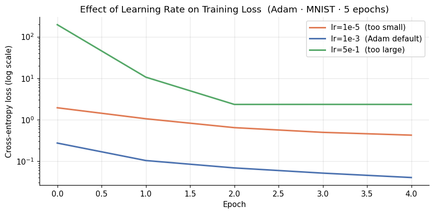
The blue run (lr=1e-3) is Adam’s default and our baseline throughout the notebook. The loss drops sharply from the first epoch onward, reaching 97.8% validation accuracy in 5 epochs.
The orange run (lr=1e-5) does converge, but much more slowly. After epoch 1 the train loss is still above 1.9, where the default is already at 0.27. It reaches 89.9% validation accuracy after 5 epochs. Given more steps it would eventually catch up, but that is exactly the point: a too-small LR wastes compute budget, and in fixed-step training regimes that budget is all you have.
The green run (lr=5e-1) never learns. The first epoch alone produces a train loss of 194, orders of magnitude above the initial random-chance value of \(\ln(10) \approx 2.3\). The model is pushed so far from any useful region that it cannot recover: all subsequent epochs hover around 2.3, with accuracy stuck near 10%.
Weight Decay: Fighting Overfitting
So far, we trained on the full 60,000 MNIST samples. The model had no opportunity to overfit: there is far more data than it can memorize.
In practice, datasets are often small relative to model capacity. When this happens, a model with enough parameters will memorize its training set. Its training loss drops toward zero, but its validation loss stagnates or rises. This gap is overfitting.
The standard remedy is L2 regularization, which adds a penalty proportional to the squared magnitude of the weights:
$$\mathcal{L}_{\text{reg}} = \mathcal{L} + \lambda \sum_i w_i^2$$
At each gradient step, this penalty pushes every weight toward zero. Smaller weights force the model to find patterns that generalize across examples rather than memorizing individual ones.
A note on AdamW. Standard Adam applies weight decay by adding \(\lambda w\) to the gradient before the adaptive scaling step. This is incorrect: the adaptive term changes the effective weight decay differently for each parameter. AdamW fixes this by applying weight decay directly to the weights, independently of the gradient update:
$$w \leftarrow w - \text{lr} \cdot \frac{\hat{m}}{\sqrt{\hat{v}} + \epsilon} - \text{lr} \cdot \lambda \cdot w$$
This decoupling is why AdamW is the standard optimizer for Transformers and most modern architectures.
In the following, we reduce the training set to 500 examples and run 20 epochs. We use wd=1.0, which is larger than production values (typically 0.01 to 0.1), but necessary here: with lr=1e-3, the effective per-step decay is lr × wd × w, and a small wd is completely invisible over a short run. The exaggerated value makes the effect unambiguous in the plots.
torch.manual_seed(42)
small_indices = torch.randperm(len(train_dataset))[:500].tolist()
small_dataset = Subset(train_dataset, small_indices)
small_loader = DataLoader(small_dataset, batch_size=32, shuffle=True)

print(f'Small train set: {len(small_dataset)} samples  |  {len(small_loader)} batches/epoch')
wd_configs = [
    (0.0, 'No weight decay'),
    (1.0, 'Weight decay  (wd=1.0)'),
]

s2_histories = {}
s2_models = {}
for wd, label in wd_configs:
    torch.manual_seed(42)
    model = MLP().to(DEVICE)
    optimizer = torch.optim.AdamW(model.parameters(), lr=1e-3, weight_decay=wd)
    print(f'\n--- {label} ---')
    s2_histories[label] = train_loop(
        model, small_loader, val_loader, optimizer, criterion, n_epochs=20
    )
    s2_models[label] = model
Epoch 1/20 | train=1.7443 | val=1.0581 | acc=0.713 | lr=1.00e-03
Epoch 2/20 | train=0.7042 | val=0.6143 | acc=0.810 | lr=1.00e-03
Epoch 3/20 | train=0.3721 | val=0.5206 | acc=0.837 | lr=1.00e-03
...
Epoch 20/20 | train=0.0029 | val=0.5188 | acc=0.871 | lr=1.00e-03
--- Weight decay (wd=1.0) ---
Epoch 1/20 | train=1.7516 | val=1.0755 | acc=0.710 | lr=1.00e-03
Epoch 2/20 | train=0.7220 | val=0.6233 | acc=0.811 | lr=1.00e-03
Epoch 3/20 | train=0.3889 | val=0.5229 | acc=0.838 | lr=1.00e-03
...
Epoch 20/20 | train=0.0115 | val=0.4306 | acc=0.874 | lr=1.00e-03
fig, ax = plt.subplots(figsize=(8, 4))
for i, (wd, label) in enumerate(wd_configs):
    ax.plot(
        s2_histories[label]['train_loss'],
        label=f'Train  ({label})',
        color=COLORS[i], linestyle='solid', linewidth=2,
    )
    ax.plot(
        s2_histories[label]['val_loss'],
        label=f'Val  ({label})',
        color=COLORS[i], linestyle='dashed', linewidth=2,
    )
ax.set_xlabel('Epoch')
ax.set_ylabel('Cross-entropy loss')
ax.set_title('Overfitting on 500 Samples  (AdamW · MNIST · 20 epochs)')
ax.legend(fontsize=8)
ax.grid(alpha=0.3)
plt.tight_layout()
plt.show()
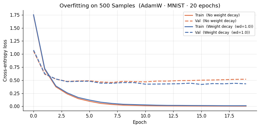
Both training curves drop to near zero by epoch 10, regardless of weight decay. The difference shows up entirely on the validation side: without regularization the validation loss plateaus around 0.52, while with weight decay it settles closer to 0.43. We can see that the weight decay consistently shifts the validation curve downward.
After training, we collect all weights across every layer and plot their distribution as a histogram. If weight decay is working, we expect the distribution to be narrower: the L2 penalty actively pushes large weights back toward zero throughout training, so no single weight should grow into an outlier.
fig, ax = plt.subplots(figsize=(8, 4))

all_weights = []
for wd, label in wd_configs:
    weights = torch.cat([
        p.detach().flatten()
        for p in s2_models[label].parameters()
    ]).cpu().numpy()
    all_weights.append(weights)
    ax.hist(
        weights, bins=80, color=COLORS[wd_configs.index((wd, label))],
        alpha=0.5, label=f'{label}  (std={weights.std():.4f})',
    )

x_max = max(abs(w).max() for w in all_weights) * 1.05
ax.set_xlim(-x_max, x_max)
ax.set_xlabel('Weight value')
ax.set_ylabel('Count')
ax.set_title('Weight Distribution After Training  (500 samples, 20 epochs)')
ax.legend()
ax.grid(alpha=0.3)
plt.tight_layout()
plt.show()
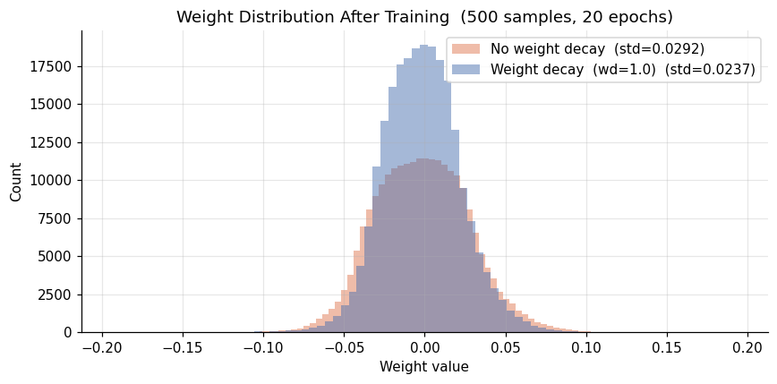
The histograms confirm the same story from the parameter side. Without weight decay, a small number of weights grow large while many others stay near zero. A few dominant weights encode specific training examples. With weight decay, no single weight becomes an outlier. The model relies on the collective contribution of many moderate weights, which generalizes better.
LR Scheduling: Adapting the Step Size Over Time
So far we have used a constant learning rate throughout training. This is suboptimal for a simple reason: the optimal step size changes as training progresses.
Early on, the loss surface is steep and the gradient points confidently toward better parameters. A larger LR is appropriate. Later, the model is near a minimum. Keeping the same LR causes the optimizer to overshoot repeatedly, and the loss oscillates rather than settling.
LR scheduling modifies the learning rate as a function of step or epoch. We look at two families of schedulers in this section.
Epoch-level Schedulers
We compare three strategies on our 500-sample subset with AdamW over 5 epochs:
- Constant: no schedule, LR stays fixed at its initial value.
- Step decay (
StepLR(step_size=2, gamma=0.3)): multiply LR by 0.3 every 2 epochs. - Cosine annealing (
CosineAnnealingLR(T_max=n_epochs)): smooth decay from initial LR to near-zero over the full run.
n_epochs = 5
s3a_configs = [
    ('Constant',         None),
    ('Step decay',       'step'),
    ('Cosine annealing', 'cosine'),
]

s3a_histories = {}
for label, sched_type in s3a_configs:
    torch.manual_seed(42)
    model = MLP().to(DEVICE)
    optimizer = torch.optim.AdamW(model.parameters(), lr=1e-3, weight_decay=1e-2)
    if sched_type == 'step':
        scheduler = torch.optim.lr_scheduler.StepLR(
            optimizer, step_size=2, gamma=0.3
        )
    elif sched_type == 'cosine':
        scheduler = torch.optim.lr_scheduler.CosineAnnealingLR(
            optimizer, T_max=n_epochs
        )
    else:
        scheduler = None
    print(f'\n--- {label} ---')
    s3a_histories[label] = train_loop(
        model, small_loader, val_loader, optimizer, criterion,
        n_epochs=n_epochs, scheduler=scheduler, batch_scheduler=False,
    )
Epoch 1/5 | train=1.7442 | val=1.0583 | acc=0.712 | lr=1.00e-03
Epoch 2/5 | train=0.7042 | val=0.6124 | acc=0.811 | lr=1.00e-03
Epoch 3/5 | train=0.3716 | val=0.5186 | acc=0.839 | lr=1.00e-03
Epoch 4/5 | train=0.2400 | val=0.4733 | acc=0.851 | lr=1.00e-03
Epoch 5/5 | train=0.1475 | val=0.4874 | acc=0.853 | lr=1.00e-03
--- Step decay ---
Epoch 1/5 | train=1.7442 | val=1.0583 | acc=0.712 | lr=1.00e-03
Epoch 2/5 | train=0.7042 | val=0.6124 | acc=0.811 | lr=1.00e-03
Epoch 3/5 | train=0.3643 | val=0.5244 | acc=0.840 | lr=3.00e-04
Epoch 4/5 | train=0.3077 | val=0.4952 | acc=0.852 | lr=3.00e-04
Epoch 5/5 | train=0.2625 | val=0.4933 | acc=0.855 | lr=9.00e-05
--- Cosine annealing ---
Epoch 1/5 | train=1.7442 | val=1.0583 | acc=0.712 | lr=1.00e-03
Epoch 2/5 | train=0.7148 | val=0.6297 | acc=0.806 | lr=9.05e-04
Epoch 3/5 | train=0.3833 | val=0.5279 | acc=0.832 | lr=6.55e-04
Epoch 4/5 | train=0.2734 | val=0.4785 | acc=0.852 | lr=3.45e-04
Epoch 5/5 | train=0.2274 | val=0.4735 | acc=0.861 | lr=9.55e-05
fig, axes = plt.subplots(1, 2, figsize=(13, 4))

ax = axes[0]
for (label, _), color in zip(s3a_configs, COLORS):
    ax.plot(s3a_histories[label]['lr'], label=label, color=color, linewidth=2)
ax.set_xlabel('Epoch')
ax.set_ylabel('Learning rate')
ax.set_title('Learning Rate per Epoch')
ax.legend()
ax.grid(alpha=0.3)

ax = axes[1]
for (label, _), color in zip(s3a_configs, COLORS):
    ax.plot(s3a_histories[label]['val_loss'], label=label, color=color, linewidth=2)
ax.set_xlabel('Epoch')
ax.set_ylabel('Cross-entropy loss (val)')
ax.set_title('Validation Loss')
ax.legend()
ax.grid(alpha=0.3)

fig.suptitle('Epoch-level LR Schedulers  (AdamW · MNIST · 5 epochs)')
plt.tight_layout()
plt.show()
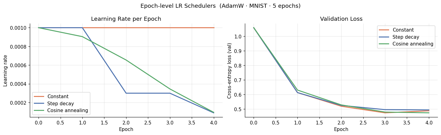
The LR plot shows the shapes clearly. Step decay follows a staircase, dropping by a factor of 0.3 every 2 epochs. Cosine annealing follows a smooth curve that approaches zero by the final epoch.
On this small setup (500 samples, 5 epochs, simple MLP), the validation loss curves are nearly indistinguishable. This is expected: scheduling effects accumulate over many epochs and are most visible on larger models and datasets. What the experiment confirms is that scheduling does not hurt, even in a regime too small to show a clear benefit.
Warmup: Handling a Cold Start
Epoch-level schedulers assume the initial LR is already appropriate from the very first step. But this is not always true.
At initialization, Adam’s second-moment estimate \(\hat{v}_t\) is zero. The bias-corrected denominator \(\sqrt{\hat{v}_t} + \epsilon\) is therefore small, and the first few update steps are abnormally large. On large models, large batches, or aggressive learning rates, these early spikes can push the model into a bad region that is hard to escape.
Warmup avoids this by starting from a very small LR and increasing it linearly over the first \(W\) steps, giving Adam time to accumulate stable variance estimates before taking full-size steps.
We combine linear warmup with cosine decay: the LR ramps from 0 to the peak over the first epoch (16 steps on our 500-sample loader), then follows cosine annealing for the remainder of training. Because this schedule operates at step resolution rather than epoch resolution, we pass batch_scheduler=True to train_loop.
n_epochs_b = 5
steps_per_epoch = len(small_loader)
total_steps = n_epochs_b * steps_per_epoch
warmup_steps = steps_per_epoch  # 1 epoch of linear warmup

def warmup_cosine_fn(step: int) -> float:
    if step < warmup_steps:
        return step / max(1, warmup_steps)
    progress = (step - warmup_steps) / max(1, total_steps - warmup_steps)
    return 0.5 * (1.0 + math.cos(math.pi * progress))

s3b_configs = [
    ('Cosine (epoch-level)', 'cosine'),
    ('Warmup + Cosine',      'warmup_cosine'),
]

s3b_histories = {}
for label, sched_type in s3b_configs:
    torch.manual_seed(42)
    model = MLP().to(DEVICE)
    optimizer = torch.optim.AdamW(model.parameters(), lr=1e-3, weight_decay=1e-2)
    if sched_type == 'cosine':
        scheduler = torch.optim.lr_scheduler.CosineAnnealingLR(
            optimizer, T_max=total_steps
        )
    else:
        scheduler = torch.optim.lr_scheduler.LambdaLR(
            optimizer, lr_lambda=warmup_cosine_fn
        )
    print(f'\n--- {label} ---')
    s3b_histories[label] = train_loop(
        model, small_loader, val_loader, optimizer, criterion,
        n_epochs=n_epochs_b, scheduler=scheduler, batch_scheduler=True,
    )
Epoch 1/5 | train=1.7503 | val=1.0774 | acc=0.716 | lr=9.05e-04
Epoch 2/5 | train=0.7256 | val=0.6507 | acc=0.802 | lr=6.55e-04
Epoch 3/5 | train=0.4024 | val=0.5319 | acc=0.834 | lr=3.45e-04
Epoch 4/5 | train=0.3040 | val=0.4954 | acc=0.856 | lr=9.55e-05
Epoch 5/5 | train=0.2687 | val=0.4941 | acc=0.854 | lr=0.00e+00
--- Warmup + Cosine ---
Epoch 1/5 | train=2.1276 | val=1.6778 | acc=0.508 | lr=1.00e-03
Epoch 2/5 | train=1.0587 | val=0.7153 | acc=0.786 | lr=8.54e-04
Epoch 3/5 | train=0.4684 | val=0.5521 | acc=0.818 | lr=5.00e-04
Epoch 4/5 | train=0.3096 | val=0.4924 | acc=0.850 | lr=1.46e-04
Epoch 5/5 | train=0.2622 | val=0.4873 | acc=0.853 | lr=0.00e+00
cosine_fn = lambda step: 0.5 * (1.0 + math.cos(math.pi * step / total_steps))
warmup_cosine_schedule = [warmup_cosine_fn(s) for s in range(total_steps)]
cosine_schedule_steps = [cosine_fn(s) for s in range(total_steps)]

fig, axes = plt.subplots(1, 2, figsize=(13, 4))

ax = axes[0]
for values, (label, _), color in zip(
    [cosine_schedule_steps, warmup_cosine_schedule], s3b_configs, COLORS
):
    ax.plot(values, label=label, color=color, linewidth=2)
ax.set_xlabel('Step')
ax.set_ylabel('LR multiplier')
ax.set_title('LR Schedule Shape  (step resolution)')
ax.legend()
ax.grid(alpha=0.3)

ax = axes[1]
for (label, _), color in zip(s3b_configs, COLORS):
    ax.plot(s3b_histories[label]['val_loss'], label=label, color=color, linewidth=2)
ax.set_xlabel('Epoch')
ax.set_ylabel('Cross-entropy loss (val)')
ax.set_title('Validation Loss')
ax.legend()
ax.grid(alpha=0.3)

fig.suptitle('Warmup + Cosine vs Cosine  (AdamW · MNIST · 5 epochs)')
plt.tight_layout()
plt.show()
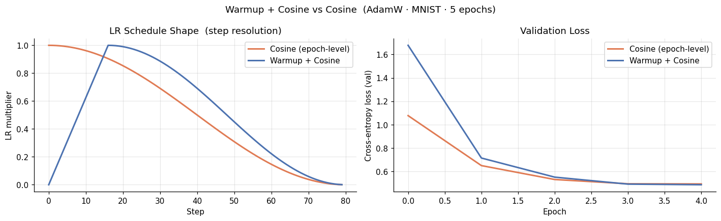
The warmup curve starts near zero and ramps up linearly over the first epoch, then follows the same cosine descent as the baseline. The two LR shapes diverge only during that initial ramp.
On our small MLP and MNIST, the difference in validation loss between the two runs is minimal. This is expected: warmup is most impactful when training is unstable at initialization, which happens with large models, large batch sizes, or large peak learning rates. For small models on simple tasks, Adam’s bias-corrected estimates stabilize quickly even without it.
If you are training a Transformer with Adam, always add warmup. The cost is near-zero and it eliminates an entire class of instabilities in the first steps.
Gradient Clipping: Surviving a Bad Batch
Even with a good learning rate and a well-tuned schedule, training can be derailed by a single anomalous batch. In practice, this happens more often than expected: a corrupted sample, an outlier with an extreme label, or a bug in the data pipeline can produce a gradient that is orders of magnitude larger than normal. The resulting parameter update overshoots, and the loss spikes.
Gradient clipping is a simple safeguard. Before the optimizer step, we rescale the gradient vector so that its global L2 norm does not exceed a threshold max_norm:
$$\text{if } |\mathbf{g}|_2 > \text{max_norm}: \quad \mathbf{g} \leftarrow \mathbf{g} \cdot \frac{\text{max_norm}}{|\mathbf{g}|_2}$$
The direction of the gradient is preserved. Only the magnitude is capped. In PyTorch this is one line placed between .backward() and .step():
nn.utils.clip_grad_norm_(model.parameters(), max_norm=1.0)
We simulate the scenario by multiplying a single batch’s inputs by 50 at step 40, after the model has already made good progress. We then compare two runs: one without clipping and one with max_norm=1.0.
corrupt_at = 40  # step 40 = epoch 3, mid-training on the 500-sample loader

def run_with_corruption(
    clip_grad: bool,
    max_norm: float = 1.0,
) -> dict[str, list[float]]:
    torch.manual_seed(42)
    model = MLP().to(DEVICE)
    optimizer = torch.optim.AdamW(model.parameters(), lr=1e-3, weight_decay=1e-2)
    step_losses, step_grad_norms = [], []
    global_step = 0
    for _ in range(5):
        model.train()
        for x, y in small_loader:
            x, y = x.to(DEVICE), y.to(DEVICE)
            if global_step == corrupt_at:
                x = x * 50.0
            optimizer.zero_grad()
            loss = criterion(model(x), y)
            loss.backward()
            step_grad_norms.append(get_grad_norm(model))
            if clip_grad:
                nn.utils.clip_grad_norm_(model.parameters(), max_norm)
            optimizer.step()
            step_losses.append(loss.item())
            global_step += 1
    return {'step_losses': step_losses, 'step_grad_norms': step_grad_norms}

s4_no_clip = run_with_corruption(clip_grad=False)
s4_clipped  = run_with_corruption(clip_grad=True)
print('Done.')
fig, axes = plt.subplots(1, 2, figsize=(13, 4))

ax = axes[0]
ax.plot(s4_no_clip['step_losses'], label='No clipping',
        color=COLORS[0], linewidth=1.5)
ax.plot(s4_clipped['step_losses'], label='Clipping (max_norm=1.0)',
        color=COLORS[1], linewidth=1.5)
ax.axvline(corrupt_at, color='#999999', linestyle='--', linewidth=1.2)
ax.text(corrupt_at + 1, 0.97, 'corrupt batch',
        transform=ax.get_xaxis_transform(), fontsize=8.5, color='#888888', va='top')
ax.set_xlabel('Step')
ax.set_ylabel('Cross-entropy loss')
ax.set_title('Per-step Loss')
ax.legend()
ax.grid(alpha=0.3)

ax = axes[1]
ax.plot(s4_no_clip['step_grad_norms'], label='No clipping',
        color=COLORS[0], linewidth=1.5)
ax.plot(s4_clipped['step_grad_norms'], label='Clipping (max_norm=1.0)',
        color=COLORS[1], linewidth=1.5)
ax.axhline(1.0, color=COLORS[1], linestyle=':', linewidth=1.2, alpha=0.6)
ax.axvline(corrupt_at, color='#999999', linestyle='--', linewidth=1.2)
ax.text(corrupt_at + 1, 0.97, 'corrupt batch',
        transform=ax.get_xaxis_transform(), fontsize=8.5, color='#888888', va='top')
ax.set_xlabel('Step')
ax.set_ylabel('Gradient L2 norm')
ax.set_title('Per-step Gradient Norm')
ax.legend()
ax.grid(alpha=0.3)

fig.suptitle('Effect of Gradient Clipping  (corrupted batch at step 40)')
plt.tight_layout()
plt.show()
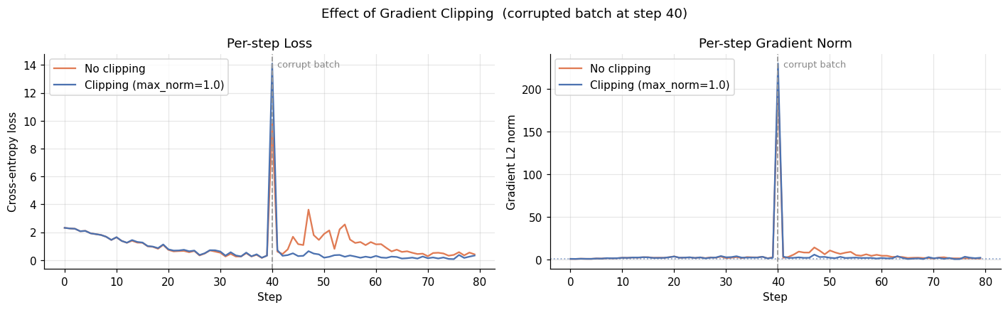
At step 40, the corrupted batch causes a sharp spike in the gradient norm. Without clipping, the norm jumps far above the normal training range and the loss visibly spikes, taking several steps to recover its previous trajectory. With clipping, both signals barely register the event: the norm is capped at max_norm=1.0 and the loss continues its downward trend.
Clipping does not prevent the corrupted batch from being processed. It ensures that no single batch can move the parameters by more than a controlled amount. In practice, max_norm values between 0.5 and 5.0 are common. The right value depends on the normal gradient scale of your model, which you can read off a clean run’s norm plot before adding any clipping.
Choosing Hyperparameters
We have now seen what each hyperparameter does: the learning rate controls step size, weight decay prevents overfitting, scheduling adapts the LR over time, and gradient clipping absorbs spikes. The remaining question is practical: given a new model and dataset, where do you start?
The answer is not a grid search from scratch. A few structured steps get you to a good configuration quickly, and the LR range test is the most useful of them.
The LR Range Test
The learning rate is the most impactful hyperparameter and the hardest to guess ahead of time. The LR range test (Smith, 2015) gives you a data-driven answer in a single short run.
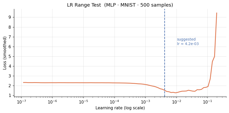
The idea is straightforward: start with a very small LR and increase it geometrically at each step, recording the smoothed loss as you go. The loss will initially decrease as the LR enters a useful range, then flatten, then rise sharply once the LR exceeds the stable region. The suggested LR is the value at the point of steepest descent, roughly one order of magnitude below where the loss starts rising.
We apply it here to our MLP on the 500-sample subset, sweeping from 1e-7 to 1.0 over 100 steps. The run stops early if the loss diverges.
def run_lr_finder(
    start_lr: float = 1e-7,
    end_lr: float = 1.0,
    num_steps: int = 100,
    smoothing: float = 0.9,
) -> tuple[list[float], list[float]]:
    torch.manual_seed(42)
    model = MLP().to(DEVICE)
    optimizer = torch.optim.AdamW(model.parameters(), lr=start_lr)
    mult = (end_lr / start_lr) ** (1.0 / num_steps)
    scheduler = torch.optim.lr_scheduler.ExponentialLR(optimizer, gamma=mult)

    lrs, losses = [], []
    avg_loss, best_loss = 0.0, float('inf')
    loader_iter = iter(small_loader)

    for step in range(num_steps):
        try:
            x, y = next(loader_iter)
        except StopIteration:
            loader_iter = iter(small_loader)
            x, y = next(loader_iter)
        x, y = x.to(DEVICE), y.to(DEVICE)
        optimizer.zero_grad()
        loss = criterion(model(x), y)
        loss.backward()
        optimizer.step()
        scheduler.step()

        avg_loss = smoothing * avg_loss + (1 - smoothing) * loss.item()
        smooth_loss = avg_loss / (1 - smoothing ** (step + 1))
        lrs.append(optimizer.param_groups[0]['lr'])
        losses.append(smooth_loss)

        if step > 10 and smooth_loss > 4 * best_loss:
            break
        best_loss = min(best_loss, smooth_loss)

    return lrs, losses

finder_lrs, finder_losses = run_lr_finder()
print(f'Range test completed over {len(finder_lrs)} steps.')
log_lrs = np.log10(finder_lrs)
slopes = np.gradient(finder_losses, log_lrs)
suggested_idx = int(np.argmin(slopes))
suggested_lr = finder_lrs[suggested_idx]

fig, ax = plt.subplots(figsize=(8, 4))
ax.plot(finder_lrs, finder_losses, color=COLORS[0], linewidth=2)
ax.axvline(suggested_lr, color=COLORS[1], linestyle='--', linewidth=1.5)
ax.text(
    suggested_lr * 2.5,
    min(finder_losses) + 0.6 * (max(finder_losses) - min(finder_losses)),
    f'suggested\nlr ≈ {suggested_lr:.1e}',
    color=COLORS[1], fontsize=9,
)
ax.set_xscale('log')
ax.set_xlabel('Learning rate (log scale)')
ax.set_ylabel('Loss (smoothed)')
ax.set_title('LR Range Test  (MLP · MNIST · 500 samples)')
ax.grid(alpha=0.3)
plt.tight_layout()
plt.show()
Practical Defaults
Once you have a good LR from the range test, the other hyperparameters have reasonable starting points.
| Hyperparameter | Default | When to change |
|---|---|---|
| Learning rate | From range test | Always run the test |
| Weight decay | 1e-2 | Lower if underfitting, higher if strongly overfitting |
| Gradient clipping | max_norm=1.0 | Adjust based on the gradient norm plot from a clean run |
| Warmup | 5% of total steps | Add when training is unstable in the first epoch |
| Schedule | Cosine annealing | Step decay if you need predictable LR drops at fixed points |
| Batch size | 128 or 256 | Scale LR proportionally when changing batch size |
LR and batch size. When you multiply the batch size by \(k\), each gradient estimate becomes more accurate, which allows a larger step. With SGD the linear scaling rule (Goyal et al., 2017) recommends scaling the LR by \(k\). With Adam, scaling by \(\sqrt{k}\) is more conservative and usually safer in practice.
Tuning order. Each hyperparameter should be tuned in isolation. Changing the LR and the weight decay at the same time makes it impossible to attribute any improvement to either one.
Hyperparameter Search
Once you have a good baseline from the range test and the defaults above, you may want to search more systematically. Three strategies are commonly used, with very different efficiency profiles.
Grid search evaluates every combination of a predefined set of values. With 3 hyperparameters and 5 values each, that is \(5^3 = 125\) runs. With 6 hyperparameters it is \(5^6 = 15{,}625\). Grid search scales exponentially and is almost never the right choice.
Random search samples each hyperparameter independently and uniformly (or log-uniformly for values that span orders of magnitude like the LR). Bergstra and Bengio (2012) showed that if only a small subset of hyperparameters actually matters, random search finds good configurations much faster than grid search. The reason is geometric: grid search wastes most of its budget evaluating redundant combinations of the unimportant ones, while random search gets more distinct values for each HP per run. In practice, 20 to 50 random trials often match or beat a dense grid.
Bayesian optimization builds a probabilistic surrogate of the objective (typically a Gaussian process or a tree-structured Parzen estimator) and uses it to decide which configuration to try next. Each trial informs the surrogate, so the search concentrates on promising regions. This is significantly more sample-efficient than random search when each trial is expensive. Optuna is the standard library for this in Python:
import optuna

def objective(trial: optuna.Trial) -> float:
    lr = trial.suggest_float('lr', 1e-5, 1e-1, log=True)
    wd = trial.suggest_float('weight_decay', 1e-4, 1e-1, log=True)
    torch.manual_seed(42)
    model = MLP().to(DEVICE)
    optimizer = torch.optim.AdamW(model.parameters(), lr=lr, weight_decay=wd)
    history = train_loop(model, small_loader, val_loader, optimizer,
                         criterion, n_epochs=5, verbose=False)
    return history['val_loss'][-1]

study = optuna.create_study(direction='minimize')
study.optimize(objective, n_trials=30)
print(study.best_params)
Not all hyperparameters are worth searching. The LR and weight decay interact directly with the loss surface and are worth tuning carefully. The schedule type, warmup length, and clipping threshold matter less and can usually be fixed at their defaults. Searching over too many dimensions dilutes the budget and makes results harder to interpret.
LR and weight decay should always be sampled on a log scale. A uniform draw over [1e-4, 1e-1] would almost never sample below 1e-3, wasting the low-LR region entirely. On a log scale, each order of magnitude gets equal coverage.
Tuning Checklist
A minimal starting procedure for a new model and dataset:
- Baseline. Train with AdamW,
lr=1e-3, no schedule, no regularization. Confirm the model can overfit the training set. If it cannot, the architecture or loss function is the problem, not the hyperparameters. - LR range test. Run the range test. Pick the LR at the point of steepest descent, roughly one order of magnitude below where the loss starts rising.
- Regularize. If validation loss diverges from training loss, add weight decay. Start at
1e-2and adjust based on the size of the gap. - Schedule. Add cosine annealing. This costs nothing and consistently helps toward the end of training.
- Warmup. Add a linear warmup over the first 5% of steps if the loss is erratic at initialization.
- Clip. Plot the gradient norm during a clean run. If it occasionally spikes far above its typical value, add
clip_grad_norm_withmax_normset to roughly the 95th percentile of the observed norm.
Each step should produce a measurable improvement. If it does not, the previous step was the binding constraint, not this one.