Gradient accumulation and KoLeo loss - Part 3/3

In the previous chapter, we observed that the KoLeo loss successfully spreads embeddings in the representation space. However, we noted that the KoLeo loss is intrinsically dependent on batch size: it computes the minimum distance between each embedding and all other embeddings within the same batch. This batch dependency naturally raises questions about the impact of gradient accumulation on training and the quality of embeddings.

What is gradient accumulation?

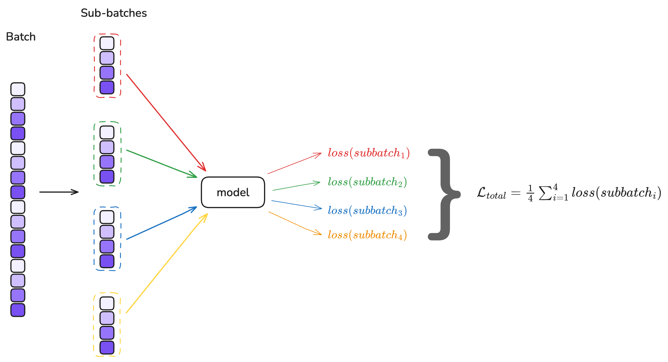
Gradient accumulation is a technique that allows training with a larger effective batch size when memory constraints limit the actual batch size that can fit in GPU memory. Instead of updating the model weights after processing a single batch, gradient accumulation processes multiple smaller batches** sequentially and then accumulates the gradients from each batch without updating the weights. It will updates the model weights only after processing all accumulated batches.

Mathematically, if we have a batch size of $B$ and accumulate gradients over $N$ batches, the effective batch size becomes $N \times B$. The loss is typically averaged over each batch, and the gradients are summed across all accumulated batches before the weight update.

Gradient accumulation illustration

For a standard loss function like the triplet loss, gradient accumulation is straightforward: the loss is computed independently for each batch, and the gradients can be safely accumulated. However, for batch-dependent losses like the KoLeo loss, the situation is more complex.

The KoLeo loss computes distances between all pairs of embeddings within a batch. When using gradient accumulation, each sub-batch computes its own KoLeo loss based only on embeddings within that sub-batch and then compute a mean of the KoLeo loss for all sub-batches. This means the KoLeo loss “sees” only the local structure within each sub-batch, not the global structure across the entire effective batch

This raises an important question: does gradient accumulation affect the behavior of the KoLeo loss, and if so, how does it impact the spread and quality of embeddings?

Gradient accumulation in action

Gradient accumulation with a standard loss (BCE loss)

To illustrate how gradient accumulation works with a standard loss like BCE lets build a small model and instantiate a loss function and an optimizer.

import torch
from torch import nn

seed = 42
torch.manual_seed(seed)
simple_model = nn.Sequential(nn.Linear(2, 3, bias=False), nn.Linear(3, 1, bias=False), nn.Sigmoid())

def print_weights(model):
    for name, param in model.named_parameters():
        print(name)
        print("-"*10)
        print(param.data.numpy())

print_weights(simple_model)

> 0.weight
> ----------
> [[ 0.5406104 0.5869042 ]
> [-0.16565566 0.6495563 ]
> [-0.15492962 0.14268756]]
> 1.weight
> ----------
> [[-0.28108588 0.3390678 0.50895905]]

Let’s run our model over all a batch of 4 samples.

loss_fn = nn.BCELoss()
batch_input = torch.randn(4, 2)
targets = torch.Tensor([0, 1, 0, 1]).unsqueeze(1)

outputs = simple_model(batch_input)
original_loss = loss_fn(outputs, targets)
print(original_loss.item())

> 0.5844024419784546

If we want to accumulate the gradients overs 4 sub-batches, each sub-batch will have 1 sample. We run the model 4 times, accumulating the loss of each sub-batch, and compute the mean loss. Here how to do it:

import copy

simple_model_gradacc = copy.deepcopy(simple_model)

grad_accum_steps = 4
sub_batch_size = len(batch_input) // grad_accum_steps
batch_losses = torch.zeros(grad_accum_steps)

for sub_batch_idx in range(grad_accum_steps):
    sub_batch_input = batch_input[(sub_batch_idx * sub_batch_size):((sub_batch_idx + 1) * sub_batch_size), ...]
    sub_batch_targets = targets[(sub_batch_idx * sub_batch_size):((sub_batch_idx + 1) * sub_batch_size), ...]

    sub_batch_outputs = simple_model_gradacc(sub_batch_input)
    sub_batch_loss_gradacc = loss_fn(sub_batch_outputs, sub_batch_targets)
    print(f"loss for sub-batch {sub_batch_idx}: {sub_batch_loss_gradacc}")

    batch_losses[sub_batch_idx] = sub_batch_loss_gradacc

loss_gradacc = batch_losses.mean()
print(f"mean loss: {loss_gradacc.item()}")

> loss for sub-batch 0: 0.5325143933296204
> loss for sub-batch 1: 0.5711992383003235
> loss for sub-batch 2: 0.7103754281997681
> loss for sub-batch 3: 0.5235207676887512
> mean loss: 0.5844024419784546

We can see that the mean loss resulting from the gradient accumulation it’s exactly the same as the loss computed from the original batch. This works, because the reduction mode of the BCELoss is mean by default.

torch.nn.BCELoss(weight=None, size_average=None, reduce=None, reduction='mean')

If we choose sum instead, we will have a total loss equal to the sum of each loss of each sample

batch_losses.sum().item()

> 2.3376097679138184

loss_sum_fn = nn.BCELoss(reduction='sum')
outputs = simple_model(batch_input)
sum_loss = loss_sum_fn(outputs, targets)
print(sum_loss.item())

> 2.3376097679138184

Ok, now let’s compute the gradients of both models, with and without gradient accumulation.

from torch.optim import SGD

def print_gradients(model):
    for name, param in model.named_parameters():
        if param.grad is not None:
            print(name)
            print("-"*10)
            print(param.grad)


optimizer = SGD(simple_model.parameters(), lr=1)
optimizer.zero_grad()
original_loss.backward(retain_graph=True)
print("Gradients of the model without gradient accumulation:")
print_gradients(simple_model)
print("="*20)

optimizer_gradacc = SGD(simple_model_gradacc.parameters(), lr=1)
optimizer_gradacc.zero_grad()

for sub_batch_idx in range(grad_accum_steps):
    sub_batch_input = batch_input[(sub_batch_idx * sub_batch_size):((sub_batch_idx + 1) * sub_batch_size), ...]
    sub_batch_targets = targets[(sub_batch_idx * sub_batch_size):((sub_batch_idx + 1) * sub_batch_size), ...]

    sub_batch_outputs = simple_model_gradacc(sub_batch_input)
    sub_batch_loss_gradacc = loss_fn(sub_batch_outputs, sub_batch_targets)
    sub_batch_loss_gradacc.backward(retain_graph=True)


print("Gradients of the model with gradient accumulation:")
print_gradients(simple_model_gradacc)

> Gradients of the model without gradient accumulation:
> 0.weight
> ----------
> tensor([[-0.1107, -0.0319],
> [ 0.1335, 0.0385],
> [ 0.2004, 0.0578]])
> 1.weight
> ----------
> tensor([[ 0.2796, 0.0086, -0.0448]])
> ====================
> Gradients of the model with gradient accumulation:
> 0.weight
> ----------
> tensor([[-0.4428, -0.1278],
> [ 0.5342, 0.1541],
> [ 0.8018, 0.2314]])
> 1.weight
> ----------
> tensor([[ 1.1185, 0.0343, -0.1792]])

The reason we see different gradient values for the model trained with and without gradient accumulation is due to how the loss is scaled in each approach.

When we process the whole batch at once (without gradient accumulation), the loss function computes the average loss over the entire batch, and backpropagation accumulates gradients based on this average.

However, when we use gradient accumulation and process the batch in smaller sub-batches, we calculate the loss (usually averaged) for each sub-batch and call .backward() on each one. This ends up accumulating the gradients for each sub-batch average rather than for the full batch average, effectively scaling the gradients by the number of accumulation steps and making them larger than expected.

To fix this we need to ensure that the overall scale of the loss matches between the two methods. The most common way to do this is to divide the loss of each sub-batch by the number of accumulation steps before calling .backward(),
In summary, when using gradient accumulation, always adjust your loss scaling to make sure gradients are computed as if you had done a single backward pass on the whole batch.

optimizer_gradacc.zero_grad()

for sub_batch_idx in range(grad_accum_steps):
    sub_batch_input = batch_input[(sub_batch_idx * sub_batch_size):((sub_batch_idx + 1) * sub_batch_size), ...]
    sub_batch_targets = targets[(sub_batch_idx * sub_batch_size):((sub_batch_idx + 1) * sub_batch_size), ...]

    sub_batch_outputs = simple_model_gradacc(sub_batch_input)
    sub_batch_loss_gradacc = loss_fn(sub_batch_outputs, sub_batch_targets) / grad_accum_steps # scale the loss by the number of accumulation steps
    sub_batch_loss_gradacc.backward(retain_graph=True)
    
print_gradients(simple_model_gradacc)

> 0.weight
> ----------
> tensor([[-0.1107, -0.0319],
> [ 0.1335, 0.0385],
> [ 0.2004, 0.0578]])
> 1.weight
> ----------
> tensor([[ 0.2796, 0.0086, -0.0448]])

We have now the same gradients, we can update our model weights to confirm we have exactly the same thing.

optimizer.step()
optimizer_gradacc.step()

print("Weights of the model without gradient accumulation:")
print_weights(simple_model)
print("Weights of the model with gradient accumulation:")
print_weights(simple_model_gradacc)

> Weights of the model without gradient accumulation:
> 0.weight
> ----------
> [[ 0.65131354 0.61885107]
> [-0.2991945 0.6110195 ]
> [-0.35537863 0.0848418 ]]
> 1.weight
> ----------
> [[-0.56070507 0.33048445 0.5537596 ]]
> Weights of the model with gradient accumulation:
> 0.weight
> ----------
> [[ 0.65131354 0.61885107]
> [-0.2991945 0.6110195 ]
> [-0.35537863 0.0848418 ]]
> 1.weight
> ----------
> [[-0.56070507 0.33048445 0.5537596 ]]

Gradient accumulation with KoLeo loss

With a standard loss function like Binary Cross Entropy (BCE), gradient accumulation is straightforward because the loss over a batch is just the mean of the losses over each individual example, and BCE is additive and independent across examples. Given a batch of predictions $\hat{y}$ and targets $y$, the total BCE loss is:

$$ \mathcal{L}_{\text{BCE}} = \frac{1}{N} \sum_{i=1}^N \ell_{\text{BCE}}(\hat{y}_i, y_i) $$

When we split a batch into sub-batches for gradient accumulation, and scale each sub-batch’s loss by $1/$ (number of accumulation steps), the overall gradients are equivalent to those computed on the full batch, because

$$ \frac{1}{K} \sum_{k=1}^K \sum_{i \in \text{sub-batch}_k}^B \frac{1}{B} \ell_{\text{BCE}}(\hat{y}_i, y_i) = \frac{1}{N}\sum_{i=1}^{N} \ell_{\text{BCE}}(\hat{y}_i, y_i) $$

where $ N = B \times K $

However, with the KoLeo loss, the situation is more complex. The KoLeo loss for a batch depends not only on individual samples, but on the distances between all possible pairs within the batch. If we split the batch into sub-batches and independently compute the KoLeo loss for each, we lose the pairwise structure across the whole batch. The result is that gradient accumulation with naive sub-batch loss scaling does not yield the same gradients as computing the KoLeo loss over the full batch.

$$ \frac{1}{K} \sum_{k=1}^K ( \frac{1}{B} \sum_{(i,j) \in \text{sub-batch}_k^2} -\log\left( \min_{j \ne i} | f(x_i) - f(x_j) | \right)) \neq \frac{1}{N}\sum_{i=1}^{N} -\log\left( \min_{j \ne i} | f(x_i) - f(x_j) | \right)) $$

We can verify this programmatically. You can find the utility scripts at https://github.com/adlane98/koleo-study.

from training_utils import KoLeoLoss

koleo_loss = KoLeoLoss()

torch.manual_seed(seed)

simple_model = nn.Sequential(nn.Linear(10, 3, bias=False), nn.Linear(3, 2, bias=False))
inputs = torch.randn(100, 10)
outputs = simple_model(inputs)
print("Loss without gradient accumulation:")
print(koleo_loss(outputs).item())

sub_batch_size = len(inputs) // grad_accum_steps
losses = torch.zeros(grad_accum_steps)
for idx in range(grad_accum_steps):
    sub_batch_inputs = inputs[(idx * sub_batch_size):((idx + 1) * sub_batch_size), ...]
    sub_batch_outputs = simple_model(sub_batch_inputs)
    sub_batch_loss = koleo_loss(sub_batch_outputs)
    losses[idx] = sub_batch_loss

print("Loss with gradient accumulation:")
print(losses.mean().item())

> Loss without gradient accumulation:
> 4.714231491088867
> Loss with gradient accumulation:
> 3.278782844543457

This example confirms that the KoLeo loss differs when computed with or without gradient accumulation. But is this a problem? In real training, can the accumulated KoLeo loss still provide a good enough approximation without breaking the training?

Integrating gradient accumulation to our code

First, we will train the same network used in chapters 1 and 2, and set the seed to ensure the training is exactly reproducible as at the beginning of chapter 2. We introduce a new hyper-parameter grad_accum_steps and we will ensure that batch_size % grad_accum_steps = 0. Moreover we make sure that the dataset length is also a multiple of the batch size so we modify the validation split to 0.0524 because 0.0524 x 25000 = 1256 so that we have 25000 - 1256 = 23744 and 23744 % 64 = 0.

import numpy as np

from training_utils import get_device, load_cifar10, build_triplets, create_datasets


seed = 42
device = get_device()
device = "cpu"
print(f"Device: {device}")

images, labels = load_cifar10("../cifar-10-python")
print(f"Images shape: {images.shape}, Labels shape: {labels.shape}")

np.random.seed(seed)
triplets, triplets_labels = build_triplets(images, labels, n_neg=2500, seed=seed)
print(f"Triplets shape: {triplets.shape}")

batch_size = 64
grad_accum_steps = 4
assert batch_size % grad_accum_steps == 0
sub_batch_size = batch_size // grad_accum_steps

learning_rate = 5e-4
margin = 0.4
koleo_weight = 0.1
val_split = 0.05

train_dataset, val_dataset, val_triplets, val_labels = create_datasets(triplets, triplets_labels, val_split=val_split, seed=seed)

koleo_loss_fn = KoLeoLoss()

print(f"Train: {len(train_dataset)}, Val: {len(val_dataset)}")

> Device: cpu
> Images shape: (50000, 32, 32, 3), Labels shape: (50000,)
> Triplets shape: (25000, 3, 32, 32, 3)
> Train: 23750, Val: 1250

We can write the new training loop, and we put the validation loop in training_utils.py because it’s the same validation loop as in Chapter 2. Note that there are several ways to implement gradient accumulation. For the sake of simplicity, we choose to do it inside the training loop and transfer the data to the device after splitting the whole batch into sub-batches, because a batch size of 64, as we’ve chosen, fits in our memory. However, in real-world scenarios, the batch size may not fit in your memory, so you would need to either change how the dataloader is implemented or use an approach like this:

optimizer = ...
NUM_ACCUMULATION_STEPS = ...

for epoch in range(...):
    for idx, sample in enumerate(dataloader):
        inputs, labels = sample

        outputs = model(inputs)
        loss = loss_fn(outputs, labels)

        loss = loss / NUM_ACCUMULATION_STEPS
        loss.backward()

        if ((idx + 1) % NUM_ACCUMULATION_STEPS == 0) or (idx + 1 == len(dataloader)):
            optimizer.step()
            optimizer.zero_grad()

We don’t use this approach because we want to maintain reproducibility in how the dataloader returns data, at least for the first run.

from tqdm import tqdm
from training_utils import triplet_loss, validation_loop

def train_loop(net, grad_accum_steps, dataloader, optimizer, margin, koleo_weight, print_freq=100):
    net.train()
    loss_accum = 0.0
    epoch_loss = 0.0
    for batch_idx, (anc, pos, neg) in tqdm(enumerate(dataloader)):

        if len(anc) < 64:
            continue
        
        optimizer.zero_grad()

        for sub_batch_idx in range(grad_accum_steps):
            anc_sb = anc[(sub_batch_idx * sub_batch_size):((sub_batch_idx + 1) * sub_batch_size), ...]
            pos_sb = pos[(sub_batch_idx * sub_batch_size):((sub_batch_idx + 1) * sub_batch_size), ...]
            neg_sb = neg[(sub_batch_idx * sub_batch_size):((sub_batch_idx + 1) * sub_batch_size), ...]

            anc_sb, pos_sb, neg_sb = anc_sb.to(device), pos_sb.to(device), neg_sb.to(device)
            anc_feat, pos_feat, neg_feat = net(anc_sb), net(pos_sb), net(neg_sb)

            t_loss = triplet_loss(anc_feat, pos_feat, neg_feat, margin)
            all_embeddings = torch.cat([anc_feat, pos_feat, neg_feat], dim=0)
            k_loss = koleo_loss_fn(all_embeddings)
            if koleo_weight is not None:
                loss = t_loss + koleo_weight * k_loss
            else:
                loss = t_loss
            
            loss = loss / grad_accum_steps
            loss_accum += loss.item()
            epoch_loss += loss.item()
            loss.backward()

        optimizer.step()


        if (batch_idx + 1) % print_freq == 0:
            print(f"Batch {batch_idx+1}: Loss = {loss_accum / print_freq:.4f}")
            loss_accum = 0.0

    return epoch_loss / (batch_idx + 1)

Setting up the training folder.

from training_utils import setup_training_dir

epochs = 15

config = {
    "seed": seed, "batch_size": batch_size, "grad_accum_steps": grad_accum_steps, "learning_rate": learning_rate,
    "epochs": epochs, "margin": margin, "koleo_weight": koleo_weight, "val_split": val_split
}
save_dir, metrics_path, csv_headers = setup_training_dir("runs_koleo_gradacc", config)

We can launch the training!

import random

from torch.utils.data import DataLoader
from torchvision.models import VGG11_Weights

from training_utils import VGG11Embedding, print_metrics, log_metrics

train_losses = []
val_losses = []
best_auc = 0
best_epoch_path = None

device = "cpu"

random.seed(seed)
np.random.seed(seed)
torch.manual_seed(seed)

if torch.cuda.is_available():
    torch.cuda.manual_seed(seed)
if torch.mps.is_available():
    torch.mps.manual_seed(seed)

gt = torch.Generator()
gt.manual_seed(seed)

val_loader = DataLoader(val_dataset, batch_size=batch_size, shuffle=False)
train_loader = DataLoader(train_dataset, batch_size=batch_size, shuffle=True, generator=gt)

net = VGG11Embedding(weights=VGG11_Weights.IMAGENET1K_V1).to(device)
optimizer = torch.optim.Adam(net.parameters(), lr=learning_rate)

val_metrics = validation_loop(net, val_loader, margin, koleo_weight, device)
print(f"Before training")
print_metrics(val_metrics)
log_metrics(metrics_path, csv_headers, 0, "", val_metrics)

for epoch_idx in range(epochs):
    train_loss = train_loop(net, grad_accum_steps, train_loader, optimizer, margin, koleo_weight)
    val_metrics = validation_loop(net, val_loader, margin, koleo_weight, device)
    val_losses.append(val_metrics['val_loss'])
    train_losses.append(train_loss)
        
    print(f"Epoch {epoch_idx+1} - train_loss: {train_loss:.4f}, val_loss: {val_metrics['val_loss']:.4f}, val_auc: {val_metrics['val_auc']:.4f}")
    print_metrics(val_metrics)
    log_metrics(metrics_path, csv_headers, epoch_idx + 1, train_loss, val_metrics)

    if val_metrics['val_auc'] > best_auc:
        best_auc = val_metrics['val_auc']
        if best_epoch_path is not None:
            best_epoch_path.unlink()
        best_epoch_path = save_dir / f'best_epoch_{epoch_idx+1}.pth'
        torch.save(net.state_dict(), best_epoch_path)
        print(f"New best AUC: {best_auc:.4f} at epoch {epoch_idx+1}")

> Before training
> Validation metrics — val_loss: 0.3296, simple_loss: 0.3156, val_auc: 0.6642, mean_positive_similarities: 0.2750, mean_negative_similarities: 0.1853, mean_positive_euclidean_distances: 1.1968, mean_negative_euclidean_distances: 1.2714, good_triplets_ratio: 0.6656
> 100it [02:19, 1.37s/it]
> Batch 100: Loss = 0.2881
> 200it [04:39, 1.36s/it]
> Batch 200: Loss = 0.2516
> 300it [06:55, 1.33s/it]
> Batch 300: Loss = 0.2195
> 372it [08:32, 1.38s/it]
> Epoch 1 - train_loss: 0.2452, val_loss: 0.2162, val_auc: 0.8650
> Validation metrics — val_loss: 0.2162, simple_loss: 0.1362, val_auc: 0.8650, mean_positive_similarities: 0.5532, mean_negative_similarities: 0.0585, mean_positive_euclidean_distances: 0.9000, mean_negative_euclidean_distances: 1.3458, good_triplets_ratio: 0.8624
> New best AUC: 0.8650 at epoch 1
> 100it [02:14, 1.34s/it]
> Batch 100: Loss = 0.1977
> 200it [04:28, 1.31s/it]
> Batch 200: Loss = 0.1752
> 300it [06:41, 1.33s/it]
> Batch 300: Loss = 0.1850
> 372it [08:15, 1.33s/it]
> Epoch 2 - train_loss: 0.1849, val_loss: 0.2147, val_auc: 0.8691
> Validation metrics — val_loss: 0.2147, simple_loss: 0.1360, val_auc: 0.8691, mean_positive_similarities: 0.5653, mean_negative_similarities: 0.0641, mean_positive_euclidean_distances: 0.8868, mean_negative_euclidean_distances: 1.3418, good_triplets_ratio: 0.8560
> New best AUC: 0.8691 at epoch 2
> 100it [02:13, 1.32s/it]
> Batch 100: Loss = 0.1640
> 200it [04:21, 1.23s/it]
> Batch 200: Loss = 0.1593
> 300it [06:26, 1.23s/it]
> Batch 300: Loss = 0.1512
> 372it [07:54, 1.28s/it]
> ...
> 100it [02:02, 1.21s/it]
> Batch 100: Loss = 0.0618
> 200it [04:04, 1.21s/it]
> Batch 200: Loss = 0.0607
> 300it [06:06, 1.21s/it]
> Batch 300: Loss = 0.0669
> 372it [07:32, 1.22s/it]
> Epoch 15 - train_loss: 0.0638, val_loss: 0.1205, val_auc: 0.9486
> Validation metrics — val_loss: 0.1205, simple_loss: 0.0729, val_auc: 0.9486, mean_positive_similarities: 0.5120, mean_negative_similarities: -0.0241, mean_positive_euclidean_distances: 0.9680, mean_negative_euclidean_distances: 1.4218, good_triplets_ratio: 0.9416
> New best AUC: 0.9486 at epoch 15

best_epoch_path = list((save_dir.glob('best_epoch_*.pth')))[0]
net.load_state_dict(torch.load(best_epoch_path))

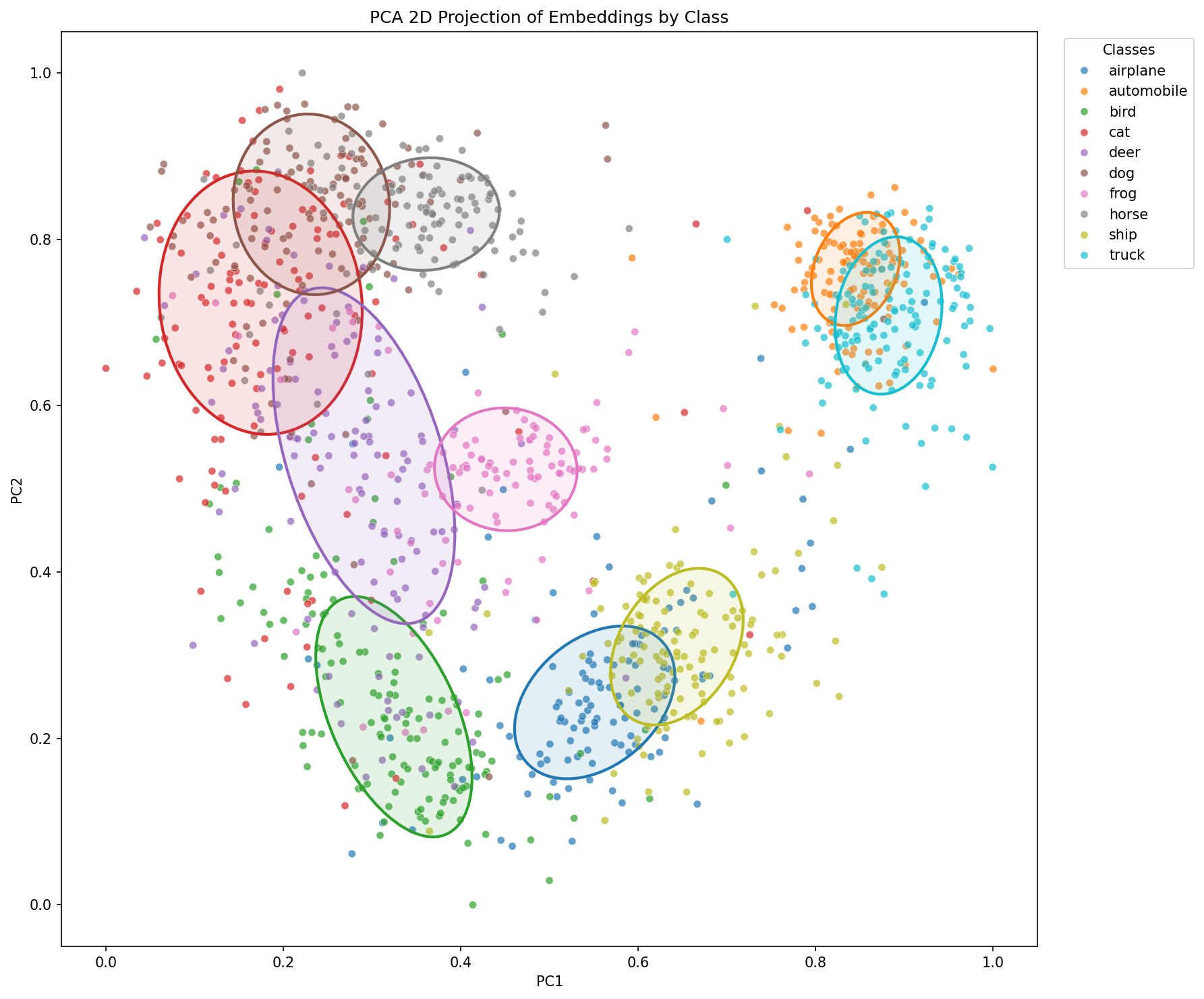
We can now compare the distance matrix and the embeddings with the ones obtained at chapter 2.

from matplotlib.patches import Ellipse
from matplotlib import pyplot as plt
import pandas as pd
import seaborn as sns

def plot_distance_matrix_and_embeddings(
    dist_matrix,
    embeddings_2d,
    ellipse_params,
    labels_array,
    label_names,
    save_path=None,
    title_suffix="",
):
    fig, axes = plt.subplots(1, 2, figsize=(20, 9))
    
    col_labels = [f"{label_names[i]}" for i in range(len(label_names))]
    row_labels = [f"{label_names[i]}" for i in range(len(label_names))]
    
    sns.heatmap(
        dist_matrix,
        xticklabels=col_labels,
        yticklabels=row_labels,
        annot=True,
        fmt='.2f',
        cmap='viridis',
        cbar_kws={'label': 'Cosine Distance'},
        ax=axes[0]
    )
    
    axes[0].set_title(f'Distance Matrix{title_suffix}', fontsize=14)
    axes[0].set_xticks(range(len(col_labels)))
    axes[0].set_xticklabels(col_labels, rotation=45, ha='right')
    axes[0].set_yticks(range(len(row_labels)))
    axes[0].set_yticklabels(row_labels, rotation=0)
    
    pca_2d_df = pd.DataFrame({
        'PC1': embeddings_2d[:, 0],
        'PC2': embeddings_2d[:, 1],
        'Label': labels_array,
        'Class': [label_names[int(label)] for label in labels_array]
    })
    
    palette = sns.color_palette("tab10", n_colors=10)
    class_names = sorted(pca_2d_df['Class'].unique())
    color_map = {cls: palette[i] for i, cls in enumerate(class_names)}
    
    sns.scatterplot(
        data=pca_2d_df, x='PC1', y='PC2',
        hue='Class', palette=color_map,
        alpha=0.7, s=30, ax=axes[1]
    )
    
    for cls in class_names:
        ep = ellipse_params[cls]
        center, w, h, angle = ep["center"], ep["width"], ep["height"], ep["angle"]
        color = color_map[cls]
        
        ellipse = Ellipse(
            xy=center, width=w, height=h, angle=angle,
            facecolor=(*color, 0.12), edgecolor=color, linewidth=2
        )
        axes[1].add_patch(ellipse)
    
    axes[1].set_xlabel('PC1')
    axes[1].set_ylabel('PC2')
    axes[1].set_title(f'PCA 2D Projection of Embeddings by Class{title_suffix}', fontsize=14)
    axes[1].legend(title='Classes', bbox_to_anchor=(1.02, 1), loc='upper left')
    
    plt.tight_layout()
    
    if save_path is not None:
        plt.savefig(save_path, dpi=150, bbox_inches='tight')
        print(f"Combined plot saved at {save_path}")
    
    plt.show()
    plt.close()
    
    same_class_dists = np.diag(dist_matrix)
    diff_class_dists = []
    for i in range(len(label_names)):
        for j in range(len(label_names)):
            if i != j:
                diff_class_dists.append(dist_matrix[i, j])
    
    print(f"\nIntra-class distance: mean={np.mean(same_class_dists):.4f}, std={np.std(same_class_dists):.4f}")
    print(f"Inter-class distance: mean={np.mean(diff_class_dists):.4f}, std={np.std(diff_class_dists):.4f}")
    print(f"Separation margin: {np.mean(diff_class_dists) - np.mean(same_class_dists):.4f}")

from matplotlib import pyplot as plt
from sklearn.decomposition import PCA

from plot_utils import compute_distance_matrix, get_ellipse_params_per_class
from training_utils import VAL_TRANSFORMS, construct_embeddings_by_class, LABEL_NAMES


embeddings_by_class = construct_embeddings_by_class(net, val_labels, val_triplets, VAL_TRANSFORMS, device)
dist_matrix = compute_distance_matrix(embeddings_by_class)

all_embeddings = torch.cat([embeddings_by_class[k] for k in embeddings_by_class], dim=0)

pca_2d = PCA(n_components=2)
embeddings_2d = pca_2d.fit_transform(all_embeddings)
embeddings_2d = (embeddings_2d - embeddings_2d.min(axis=0)) / (embeddings_2d.max(axis=0) - embeddings_2d.min(axis=0))
samples_per_class = [len(embeddings_by_class[i]) for i in range(10)]

labels_array = np.concatenate([np.full(count, label) for label, count in enumerate(samples_per_class)])
ellipse_params = get_ellipse_params_per_class(embeddings_2d, labels_array, LABEL_NAMES, coverage=0.5)

plot_distance_matrix_and_embeddings(dist_matrix, embeddings_2d, ellipse_params, labels_array, LABEL_NAMES, save_path=save_dir / "distance_matrix_and_embeddings_gradacc.png")

> Combined plot saved at runs_koleo_gradacc/20251230_131112/distance_matrix_and_embeddings_gradacc.png

png

> Intra-class distance: mean=0.4854, std=0.0488
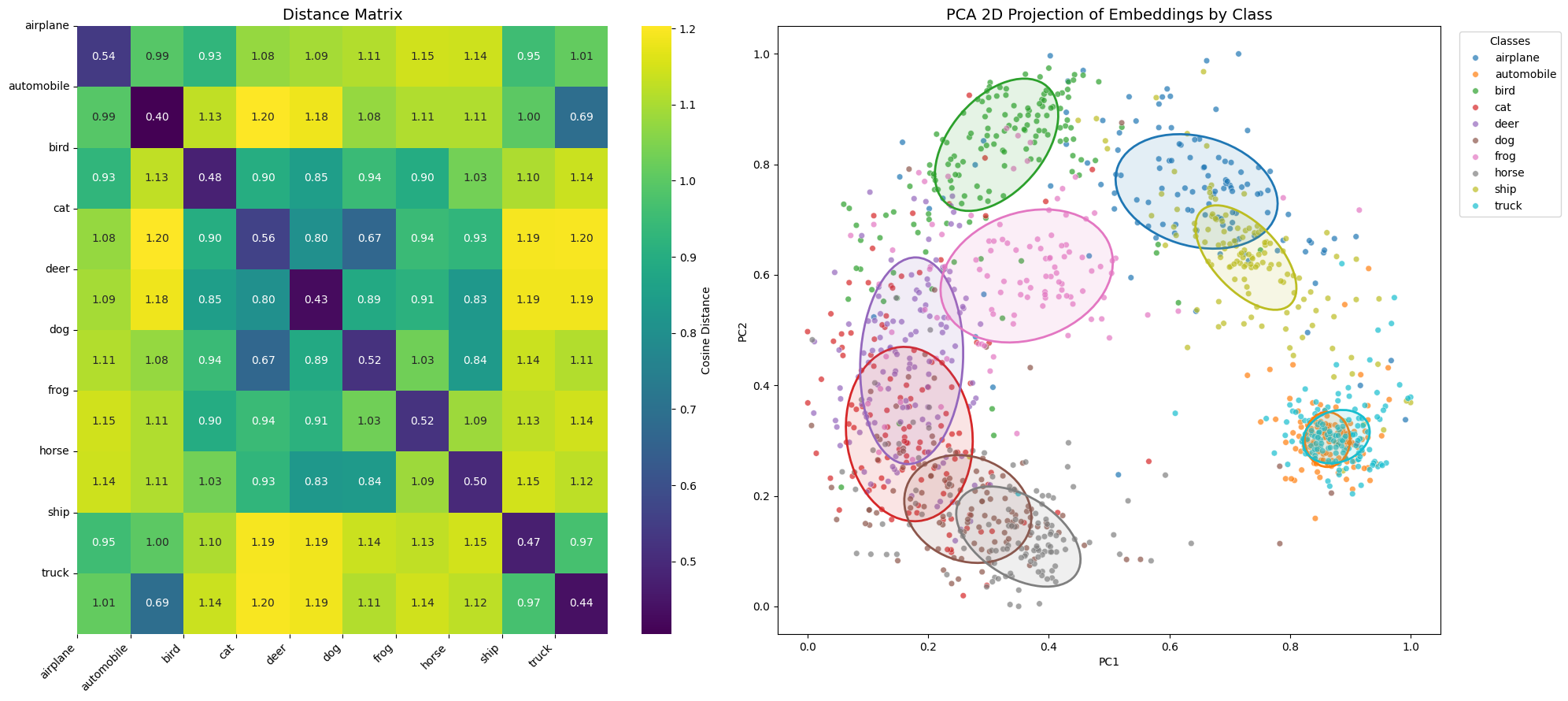
> Inter-class distance: mean=1.0279, std=0.1357
> Separation margin: 0.5425

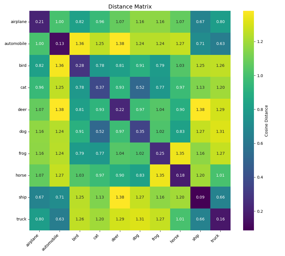
Here a table summarizing result we got in the two previous chapters.

Metric	Without KoLeo	With KoLeo	With KoLeo and gradient accumulation
Intra-class distance	mean=0.2249, std=0.0865	mean=0.5202, std=0.0545	mean=0.4854, std=0.0488
Inter-class distance	mean=1.0392, std=0.2285	mean=1.0350, std=0.1244	mean=1.0279, std=0.1357
Separation margin	0.8143	0.5147	0.5425

With gradient accumulation, the results seem to be equivalent to training with only KoLeo, but it’s too early to draw such a conclusion. To confirm this, we will perform a new K-Fold training.

K-Fold training

First, we will initialize the K-Fold training. We also choose the number of negative samples to keep when building the triplets dataset to ensure that every batch, even the last one, contains exactly 64 samples. Indeed, if we keep 2500 negative samples, we would have 25000 samples total, and 25000 * 0.95 = 23750 samples for training. However, with 23750 samples and a batch size of 64, the last batch will contain only 6 samples, because 23750 % 64 = 6. Since we have gradient accumulation steps of 4, each sub-batch will contain 16 triplets, except for the last 4 sub-batches. The first of those 4 will contain 6 samples, and the next ones 0 because there are no more triplets. There are not enough triplets in the last batch.

import numpy as np
from training_utils import build_triplets,load_cifar10
images, labels = load_cifar10("../cifar-10-python")

np.random.seed(seed)
triplets, triplets_labels = build_triplets(images, labels, n_neg=2432, seed=seed)
print(triplets.shape)

> (24320, 3, 32, 32, 3)

from sklearn.model_selection import KFold

import copy

K_FOLDS = 5
EPOCHS_PER_FOLD = 7

kfold = KFold(n_splits=K_FOLDS, shuffle=True, random_state=seed)

device = get_device()

results_no_gradacc = {"areas": {cls: [] for cls in LABEL_NAMES}, "auc": []}
results_with_gradacc = {"areas": {cls: [] for cls in LABEL_NAMES}, "auc": []}

from training_utils import train_and_compute_metrics

for fold_idx, (train_idx, val_idx) in enumerate(kfold.split(triplets)):
    print(f"\n{'='*50}")
    print(f"Fold {fold_idx + 1}/{K_FOLDS}")
    print(f"{'='*50}")
    
    fold_train_triplets = triplets[train_idx]
    fold_val_triplets = triplets[val_idx]
    fold_train_labels = triplets_labels[train_idx]
    fold_val_labels = triplets_labels[val_idx]
    
    print(f"Training WITHOUT gradient accumulation...")
    metrics_no_gradacc = train_and_compute_metrics(
        fold_train_triplets, 
        fold_val_triplets, 
        fold_val_labels,
        epochs=EPOCHS_PER_FOLD, 
        koleo_weight=0.1, 
        grad_accum_steps=4, 
    )
    for cls in LABEL_NAMES:
        results_no_gradacc["areas"][cls].append(metrics_no_gradacc["areas"][cls])
    results_no_gradacc["auc"].append(metrics_no_gradacc["auc"])
    print(f"  Best AUC: {metrics_no_gradacc['auc']:.4f}")
    
    print(f"Training WITH gradient accumulation...")
    metrics_with_gradacc = train_and_compute_metrics(
        fold_train_triplets, 
        fold_val_triplets, 
        fold_val_labels,
        epochs=EPOCHS_PER_FOLD, 
        koleo_weight=0.1, 
        grad_accum_steps=1, 
    )
    for cls in LABEL_NAMES:
        results_with_gradacc["areas"][cls].append(metrics_with_gradacc["areas"][cls])
    results_with_gradacc["auc"].append(metrics_with_gradacc["auc"])
    print(f"  Best AUC: {metrics_with_gradacc['auc']:.4f}")
    
    print(f"Fold {fold_idx + 1} done.")

> ==================================================
> Fold 1/5
> ==================================================
> Training WITHOUT gradient accumulation...
>
> 100%|█████████████████████████████████████████████████████████████████████████████████████████████████████████████████| 7/7 [05:55<00:00, 50.82s/it]
>
> Best AUC: 0.9135
> Training WITH gradient accumulation...
>
> 100%|█████████████████████████████████████████████████████████████████████████████████████████████████████████████████| 7/7 [04:03<00:00, 34.83s/it]
>
> Best AUC: 0.9149
> Fold 1 done.
> ...
> ==================================================
> Fold 5/5
> ==================================================
> Training WITHOUT gradient accumulation...
>
>
> 100%|█████████████████████████████████████████████████████████████████████████████████████████████████████████████████| 7/7 [05:50<00:00, 50.04s/it]
>
>
> Best AUC: 0.9215
> Training WITH gradient accumulation...
>
>
> 100%|█████████████████████████████████████████████████████████████████████████████████████████████████████████████████| 7/7 [04:36<00:00, 39.54s/it]
>
>
> Best AUC: 0.9111
> Fold 5 done.

Results

As in Chapter 2, we analyze the results from the K-Fold cross-validation by comparing the AUC scores and ellipse areas between the two conditions: training without gradient accumulation and training with gradient accumulation.

auc_no_gradacc = np.array(results_no_gradacc["auc"])
auc_with_gradacc = np.array(results_with_gradacc["auc"])

print("=" * 70)
print("AUC SCORES")
print("=" * 70)
print(f"Without gradient accumulation: {auc_no_gradacc.mean():.4f} +/- {auc_no_gradacc.std():.4f}")
print(f"With gradient accumulation: {auc_with_gradacc.mean():.4f} +/- {auc_with_gradacc.std():.4f}")

print("\n" + "=" * 70)
print("ELLIPSE AREAS")
print("=" * 70)
print(f"{'Class':<12} | {'Without KoLeo (mean +/- std)':<25} | {'With KoLeo (mean +/- std)':<25}")
print("-" * 70)

for cls in ["cat", "dog", "horse", "ship"]:
    no_gradacc_arr = np.array(results_no_gradacc["areas"][cls])
    with_gradacc_arr = np.array(results_with_gradacc["areas"][cls])
    
    print(f"{cls:<12} | {no_gradacc_arr.mean():.4f} +/- {no_gradacc_arr.std():.4f}        | {with_gradacc_arr.mean():.4f} +/- {with_gradacc_arr.std():.4f}")

print("\n" + "=" * 70)
print("Average area across all classes:")

all_no_gradacc = np.array([np.mean(results_no_gradacc["areas"][cls]) for cls in LABEL_NAMES])
all_with_gradacc = np.array([np.mean(results_with_gradacc["areas"][cls]) for cls in LABEL_NAMES])

print(f"  Without gradient accumulation: {all_no_gradacc.mean():.4f} +/- {all_no_gradacc.std():.4f}")
print(f"  With gradient accumulation: {all_with_gradacc.mean():.4f} +/- {all_with_gradacc.std():.4f}")

> ======================================================================
> AUC SCORES
> ======================================================================
> Without gradient accumulation: 0.9193 +/- 0.0037
> With gradient accumulation: 0.9177 +/- 0.0056
>
> ======================================================================
> ELLIPSE AREAS
> ======================================================================
> Class | Without KoLeo (mean +/- std) | With KoLeo (mean +/- std)
> ----------------------------------------------------------------------
> cat | 0.2119 +/- 0.0773 | 0.2169 +/- 0.0473
> dog | 0.1369 +/- 0.0475 | 0.1217 +/- 0.0358
> horse | 0.1474 +/- 0.0399 | 0.1438 +/- 0.0415
> ship | 0.0944 +/- 0.0272 | 0.0856 +/- 0.0233
>
> ======================================================================
> Average area across all classes:
> Without gradient accumulation: 0.1479 +/- 0.0633
> With gradient accumulation: 0.1464 +/- 0.0581

from plot_utils import plot_auc_and_ellipse_areas

plot_auc_and_ellipse_areas(
    results_no_gradacc,
    results_with_gradacc,
    ["Without GA", "With GA"],
    LABEL_NAMES,
)

png

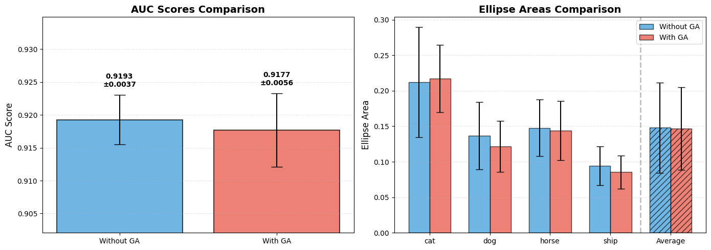
The K-Fold cross-validation results provide strong statistical evidence that gradient accumulation does not significantly degrade the performance of models trained with the KoLeo loss. The small difference between the two AUC scores falls well within the standard deviations, indicating that the discrimination ability of the model remains essentially unchanged.

Similarly, the ellipse areas show remarkable consistency across both training strategies, demonstrating that the spread of embeddings in the representation space is preserved. This finding is particularly important because it suggests that even though the KoLeo loss is computed independently on each sub-batch during gradient accumulation, the accumulated effect still achieves the desired regularization objective of spreading embeddings uniformly.

Conclusion

In this chapter, we investigated the impact of gradient accumulation on the KoLeo loss, a batch-dependent regularization technique. We began by demonstrating that gradient accumulation fundamentally changes how the KoLeo loss is computed: when a batch is split into sub-batches, each sub-batch computes its own KoLeo loss based only on the embeddings within that sub-batch, rather than considering the global structure across the entire effective batch.

Through a single training run, we observed that models trained with gradient accumulation produced embeddings with similar characteristics to those trained without it, suggesting that the approximation might be sufficient for practical purposes. To validate this observation statistically, we performed a 5-fold cross-validation experiment comparing both training strategies.

The K-Fold results confirmed our initial observation: gradient accumulation does not significantly impact either the discrimination quality (AUC scores) or the spread of embeddings (ellipse areas). This demonstrates that the local structure captured within each sub-batch during gradient accumulation is sufficient to maintain the beneficial effects of the KoLeo loss.

Synthesis of the series

This series has explored siamese networks trained with triplet loss and KoLeo regularization, examining both the theoretical foundations and practical implications of batch-dependent losses.

We began by establishing a baseline (Chapter 1), training a Siamese network with triplet loss alone on CIFAR-10. The model learned to separate classes in the embedding space with good discrimination quality and clear visual separation, as shown in distance matrices and PCA projections, though embeddings formed compact intra-class clusters.

Building on this foundation, we introduced the KoLeo loss as a regularization technique to encourage a more uniform distribution of embeddings (Chapter 2). Through K-Fold cross-validation, we confirmed that the KoLeo loss achieves its objective: embeddings spread more uniformly in the representation space, with ellipse areas increasing. We also investigated the effect of the KoLeo loss weight parameter, revealing a clear trade-off between embedding spread and discrimination quality.

Finally, we addressed a critical practical concern: the impact of gradient accumulation on the batch-dependent KoLeo loss (Chapter 3). While gradient accumulation fundamentally changes how the KoLeo loss is computed—processing sub-batches independently rather than considering the full batch—we demonstrated through K-Fold validation that the practical impact is negligible. Both AUC scores and embedding distributions remain essentially unchanged when using gradient accumulation, validating its use in memory-constrained scenarios.

Together, these three chapters provide a complete picture of how to effectively use the KoLeo loss in practice. The loss successfully spreads embeddings while maintaining discrimination quality, and it can be safely combined with gradient accumulation when needed. Although the batch-dependent nature of the loss is theoretically important, it does not prevent its practical application in real-world training scenarios.

Next steps

The very goal of this study was not to find the best model, but to demonstrate the effect of the KoLeo loss and the impact of gradient accumulation. Nevertheless, it’s interesting to consider what the best model might look like.

Throughout our experiments, we chose fixed values for the learning rate (5e-4), margin (0.4), and KoLeo weight (0.1) based on preliminary testing, rather than through thorough optimization. Although we have shown that the KoLeo loss works well and is compatible with gradient accumulation, the question of optimal hyperparameter choices remains open.

As a logical next step, it would be valuable to carry out a systematic hyperparameter search to identify the best configuration for maximizing the AUC score, with or without KoLeo Loss, with or without gradient accumulation.